Terrestrial laser scanning (TLS) is a fast, effective method for the collection of three-dimensional data. It has in the meantime also become established as a suitable alternative method for the measurement of trees in forests. Its practical application in forestry in the past was considered to be limited by the lack of a software (processing tool), that could more or less automatically derive dendrometric parameters from the large TLS datasets.
In 2017, the 3D Forest software (https://www.3dforest.eu ) was developed to do just that as part of an EU-funded project. This software has been used at the Bavarian State Institute of Forestry (LWF) ever since as a standard tool for the preliminary evaluation of TLS data. Although the software has already reached a high standard, as far as its user-friendliness and the quality of its results are concerned, even just studying the associated documentation is very time-consuming for anyone wishing to become familiar enough with the software’s use to actually work efficiently.
This article is thus a bit like a “recipe”, providing step-by-step instructions on how to use the software to extract relevant parameters quickly from point cloud data provided by the TLS data. We use data from the forest climate station in Altdorf near Nuremberg as an example showing one possible evaluation path. The results are then compared with the results of the full terrestrial survey taken in the autumn of 2019. Interested parties are welcome to request this data from the author for their own practising purposes.
Data collection in the field
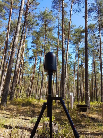
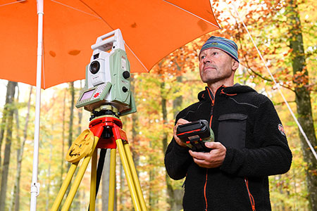
The TLS measurements were made on 08.05.2020, using the Leica BLK 360 terrestrial laser scanner, which is a lightweight device (<1 kg), with a relatively short range (60 m). On the area of the Altdorf forest climate station, the device was set up nine times along an axis drawn between the climate station’s rain collectors (Fig. 1).
The intensively measured area of the forest climate station is 50 m x 50 m in size, and it is a pure stand stocked with 110-year old pines. Although the device can in principle register the individual scan positions in relation to each other, experiences to date have shown that the automatic registration of the BLK 30 only works without error in the forest when used with very short distances of just a few metres between the scan positions. For this reason, three reference points were provided between the set-up positions to allow for a quick rough orientation and for manual registration (stitching) of the scan set-ups in relation to one another.
The LWF uses yellow, blue and red foam balls as reference points, set up across the recording area. The 360° panoramic scans were remote controlled using an iPad and the Autodesk Recap mobile app. The field survey took a total of just under two hours.
Evaluation using 3D Forest
The 3D Forest software was developed as part of an EU-funded project and has been available for free download via the URL www.3dforest.eu for Microsoft Windows (10)-based operating systems since 2017.
First of all, the software is installed using the appropriate installation file. Once the program has been started successfully, two windows (user interface and associated server application) appear. The following steps in the process are crucial for the evaluation of the TLS-measurements using 3D Forest:
1) Create project
First of all, create a new project in the user interface by clicking on “Project - New project” in the menu bar. In the “Project manager” dialogue box that now opens, you need to create a project name and a directory for the storage of project files. Then a window appears, in which a transformation matrix or an already created matrix can be loaded. In the simplest case, we select the setting “NO_MATRIX” under the option button “Choose transform matrix”, and confirm the selection. This means the XYZ-coordinates of the measurement will be used by default.
(2) Data import and visualisation
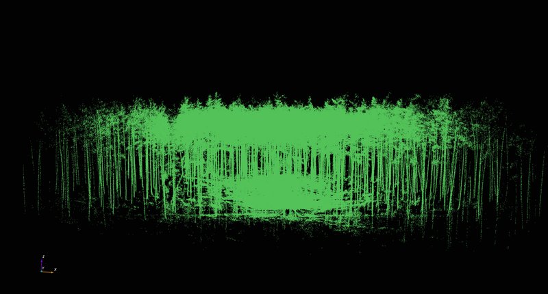
In the following step, you import the TLS raw data into the created project by clicking on “Project - Import - Import base cloud” on the menu bar. At the LWF, the original scan data and an export in the form of a text file (PTS) are saved by default. The evaluations are carried out generally on the basis of the PTS-file. During its application to date, it has been observed that 3D Forest often aborts the import of very large files. To make it basically possible to work with very large input files, scientists at the LWF have created an R-function that reduces the size of huge files by taking into account only every “nth” dataset. For the evaluation presented here, the original file of around 2.4 gigabytes was reduced to around 500 megabytes by considering only every fifth dataset. The result of the import is shown in Fig. 3. The three-dimensional data can be viewed from different angles by dragging with the mouse or by holding down the Strg/Crtrl key and dragging with the mouse at the same time. By holding down the shift key, you can move the point cloud generally within the screen section. You can use the rotating middle button on the mouse to zoom in and out.
(3) Segmentation of terrain and vegetation data
Once the data has been imported, the underlying dataset is divided into ground surface data points and vegetation data points. In principle, we can try to separate out the point clouds using Voxel cells or OCTree. We found the OCTree recognition worked well. This can be selected in the menu bar via “Terrain - Terrain from octree”. Based on our experiences to date, it is helpful to set the standard value in the dialogue window “Terrain created with octree” from the default 10 cm to values between 30 cm and 50 cm. For this evaluation, we selected 50 cm. 3D Forest divides up the dataset according to potential ground points (Terrain_octree.pcd) and according to vegetation points (Vegetation_octree.pcd). Where there are larger gaps in the ground data, a ground surface can alternatively be generated using modelling data (inverse distance weighting) to interpolate the missing terrain, thus filling the gaps, by clicking on “IDW” in the “Terrain” menu. This also worked very well.
(4) Cleaning up the “terrain point cloud”
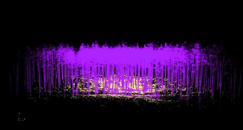
In use of this technology up to now, it has always been necessary to clean up the terrain point cloud by removing points that do not represent the terrain. The clean-up can be started via “Terrain - Manual adjustment” in the menu bar. Once the “terrain point cloud” (Terrain_octree.pcd) has been selected, it can be moved around within the view using the mouse and keyboard as described in the previous section. By clicking on Shift+X, you can switch to the mode for deleting data points. To clean-up the terrain point cloud we found it works well if you select the side view on to the point cloud. If you then switch to the “deletion mode” (Shift+X), you can remove the “ground noise” by “dragging” the relevant two-dimensional sections. By clicking on “Stop EDIT”, you save the cleaned up terrain point cloud under Terrain_octree.pcd and the deleted ground points under Terrain_rest.pcd. The results of the segmentation of the point cloud for Altdorf forest climate station according to terrain points (cleaned up) and vegetation points are presented in Fig. 4.
(5) Single tree segmentation
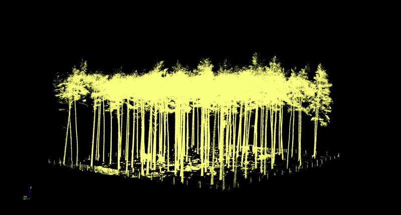
In the next step in the process, the “Vegetation point cloud” (Vegetation_octree.pcd) is segmented according to individual trees. It proved useful to trim the area in which the trees to be evaluated are in advance, i.e. remove outlying data points first. This can be done by selecting “Vegetation - Manual tree selection” from the menu list. This is as described in Section (4) Cleaning up the “terrain point cloud” using X + Shift. By clicking on “Stop EDIT”, you stop the process, and the trees that have not been deleted are saved under Tree.pcd. In the case of the Altdorf forest climate station, we removed the points outside the boundary fence, which is clearly visible in the point cloud. The result is a point cloud called "Vegetation_tree.pcd" and a point cloud called "Vegetation-rest.pcd".
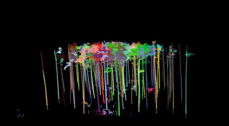
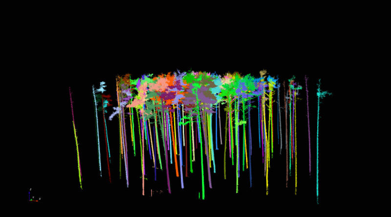
The former shows the results of the trimmed point cloud (Fig. 5) before it is segmented further into individual trees. The further segmentation is done by clicking on “Vegetation - Automatic tree segmentation” in the menu bar. It proved useful to adjust the default settings in the “Automatic segmentation” dialogue box and to go to the “Input distance” field and then change the values for “input range in %”. For the Altdorf forest climate station, values of 5 m and 60 % were selected. Once the input is confirmed, individual point clouds are created for each individual segmented tree and transferred into the project. The checking of the results proved extremely time-consuming, as the results of the automated segmentation had to be checked visually. Where necessary, each individual tree had to be removed singly by marking it with the left mouse button and then confirming the removal with the right mouse button. Figure 6 shows the results of the automated segmentation for the area in Altdorf. Fig. 6a includes misclassifications. These are eliminated in a time-consuming and labour-intensive further step by deactivating the tree group and visually inspecting each individual object. Misclassified objects are removed from the overall dataset (by selecting with the left mouse button, removing with the right mouse button, and then confirming with left mouse button).
(6) Determination of dendrometric parameters
In the next step in the process, dendrometric parameters are determined at individual tree level for the segmented tree objects. For this purpose, you determine the lowest point of each tree relative to its z-coordinate. This is done via the menu bar by clicking on “Trees - Position lowest point” or “Trees - Position RHT” (tree base position computed by randomised Hough transformation).
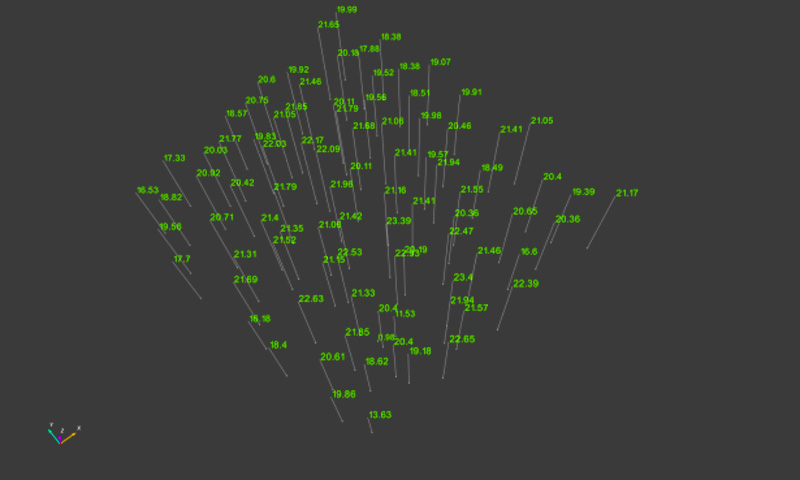
Up to now, the best results have been achieved by choosing the first of these options. This step should also be carried out at individual tree level, as it has been shown that the selection of several tree objects at the same time in the “Compute tree position using [...]” dialogue box often leads to the program crashing. This step is made somewhat easier if misclassified objects are removed in advance from the tree list as described above, and the “Input Tree Cloud” list only contains valid tree objects. Once the lowest tree positions have been determined, experience to date has shown that the other parameters (e.g. BHD or height calculation) can be calculated for all tree objects together by using the relevant multiple selection option. Once the calculations at single tree level have been completed, the values can be exported in tabular form as a txt-file by clicking on “Trees - Export Tree Parameters” on the menu bar, and processed further with external software where applicable. Graphic outputs can be generated to show the individual calculated parameters, shown in Figure 7 below using the height measurement values determined as an example.
Results for the Altdorf forest climate station
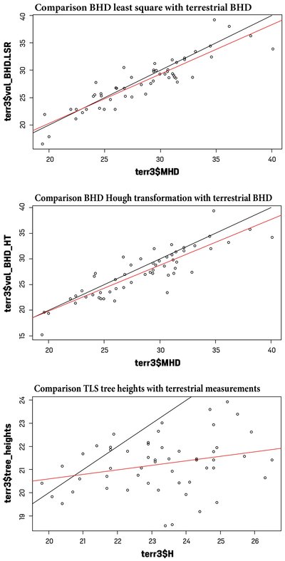
Fig. 8: Comparison of dendometric parameters obtained from traditional field surveys and terrestrial laser scan data at the Altdorf forest climate station. Shown at the top and in the middle are the BHD values obtained using least square regression (LSR) and Hough transformation (HT) respectively. In the bottom graph, the height values determined using 3D Forest are compared with the height values obtained during the full terrestrial survey of the year 2019 (H).
Figure 8 shows the comparisons of the automatically derived parameters for breast height diameter (BHD) and tree heights. For BHD, both the values derived using circle fitting (least square regression, Fig. 8 top) and those derived using Hough transformation (Fig. 8 middle) are compared. It can be seen that with both derivation methods at the individual tree level, there are in some cases considerable deviations of up to 3 cm between the TLS survey and the terrestrial survey. By contrast, the mean values of 27.33 cm for Hough transformation-BHD values and 27.87 cm for circle fitting-BHD values are relatively close to the value of 28.42 cm determined in the terrestrial survey. The results of the Mann-Witney-U test reveal no significant differences between the terrestrial data and the data derived using the TLS. In the bottom graphic in Figure 8, the values of the tree heights derived from the TLS are compared with those collected in the terrestrial survey. A significant discrepancy can be seen, especially in the larger height measurements. This is also confirmed by the comparisons of the mean and median values. Whereas the mean height value for the forest climate station in Altdorf was 23.27 m in the terrestrial survey, it was 21.23 m when derived from TLS data. The differences in the medians of the distributions were statistically validated.
The evaluation method shown here initially took approx. 3 to 4 hours. This was before the scientists were well practised in use of the technology. In the meantime, we require a maximum of one hour for evaluations of the described scope (from reading of the data to production of a table with dendrometric parameters).
Discussion and outlook
What we have described here is one way of determining dendrometric parameters from TLS data using the free software 3D Forest. While the BHD values derived automatically from the TLS data correlate well with the BHD values established in terrestrial surveys, there were large differences in the comparison between the two determining systems when it came to tree height. This confirms the findings of other studies, which also report a tendency for tree heights derived using TLS technology to be underestimated.
It appears possible in principle to derive dendrometric parameters quickly and efficiently with the help of terrestrial laser scanning data and the standard software 3D Forest, although there is still room for refinement and optimisation of the method in many ways. Our aim here was to describe a quick, foolproof method to enable people to use the 3D Forest software quickly and accurately. The article thus offers a simple description of the procedure, offering a sort of “recipe” for the software’s use.
It should be borne in mind that the application presented here was for a simple stand situation (single-layer, pure stand with one tree species). In the case of stands with more complex structures, experience to date shows that the use of 3D Forest can lead to problems that are not described here.
Furthermore, the fact that the TLS was set up on just one line must be viewed critically. This approach was not very expedient and must be changed or optimised for future applications. It should also be noted that, with the current level of development, we can only expect a partially automated analysis to be possible with 3D Forest. The individual interim steps described all require a visual inspection of the quality of the result achieved. One important wish for the future is for an automatic classification of the tree species in the 3D point clouds to be added to 3D Forest.
The authors would be delighted to exchange experiences and welcome any ideas or suggestions for improvements in the handling of 3D Forest.

